
Examples / TI op amp handbook / Integrators
Double integrator
SBOA092B page 58, Double Integrator: two T networks and one op amp (a TLC265x). The input T is RI, RI (1 MΩ each) with CI (1 µF) from their junction to ground. The feedback T is CO, CO (1 µF each) with RO (10 kΩ) from their junction to ground.
E_O = -4/(R_I C_I)² ∬ E_I dt = -4 ∬ E_I dt, where C_O = C_I/2, R_O = R_I/2The circuit
Section titled “The circuit”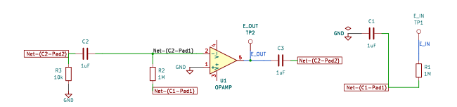
The schematic is drawn by copperhead’s
drafting engine from this circuit’s netlist, with KiCad’s own library symbols,
and it opens in KiCad as figure/double_integrator.kicad_sch.
The op amp is KiCad’s generic one, since the handbook’s are ideal, and each
terminal is a test point named as the program names it. KiCad reads back from
the sheet exactly the connections the circuit has; draw_figures.py refuses to write
one that does not.
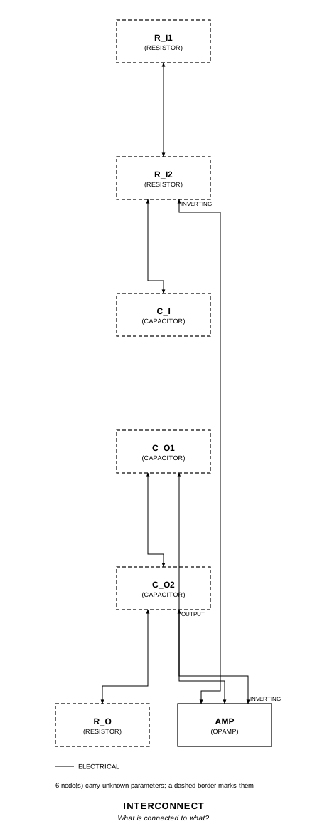
The interconnect view is fang’s own projection. It names the parts as the program does, so it reads against the code below.
What the program says
Section titled “What the program says”Working the two tees as transfer admittances gives
E_O/E_I = -(1 + 2p C_O R_O) / (R_I (2 + p R_I C_I) p² C_O² R_O)With the page’s rule the two first-order factors cancel and the transfer is
exactly -4/(p R_I C_I)². The drawn values do not follow the rule, though
(1 µF and 10 kΩ where it asks for 0.5 µF and 500 kΩ). The program keeps the
drawn values (reading) and claims what they give:
k_drawn = -1/(2 R_I R_O C_O²) = -50 /s² at low frequency. It holds the
rule’s values as parameters (c_o_rule, r_o_rule) and the printed
coefficient as k_rule = -4 /s².
The rule’s circuit is simulated as a copy written in raw cards beside the
drawn one. The bench can override parameters only on the parts it writes
itself, and fang writes the resistors and capacitors. The op amp gets 140 dB
of open-loop gain (op_amp). The circuit has no DC feedback, and at 120 dB
the low-frequency coefficient comes out 1.2% high.
What the simulation found
Section titled “What the simulation found”out/simulation.txt, from the decks under out/spice/:
| Run | Measured | Claimed |
|---|---|---|
drawn, -|E_O/E_I| (2π f)² at 10 mHz | -50.04 /s² | -50 /s² (k_drawn), holds |
drawn, gain at 0.1 Hz | 120.8 | 120.84, holds (the rule would give 10.13) |
drawn, gain at 1 Hz | 0.3872 | 0.38717, holds (the rule would give 0.1013) |
rule, -|E_O/E_I| (2π f)² at 0.1 Hz and 1 Hz | -4 /s² | -4 /s² (k_rule), holds |
rule, phase at 1 Hz | 0 rad | 0, holds |
rule_step, 0.1 V step, E_O at 2 s over (0.1 × 2²/2) | -4 /s² | -4 /s² (k_rule), holds |
Where the handbook is off
Section titled “Where the handbook is off”The drawn C_O (1 µF) and R_O (10 kΩ) do not satisfy the page’s own C_O = C_I/2, R_O = R_I/2. As drawn, the circuit double-integrates at low frequency with a coefficient of 50, not 4. Above 0.3 Hz the input T’s pole adds a third integration. The printed -4 ∬ E_I dt holds with C_O = 0.5 µF and R_O = 500 kΩ.
Running it
Section titled “Running it”fang check examples/ti_opamp_handbook/integrators/double_integrator/double_integrator.pypython examples/regenerate.py ti_opamp_handbook/integrators/double_integrator # needs ngspiceThe whole program
Section titled “The whole program”"""The double integrator, SBOA092B page 58 (bottom).Show 31 more lines
E_O = -4/(R_I C_I)^2 double integral E_I dt = -4 double integral E_I dt, where C_O = C_I/2 and R_O = R_I/2
Two T networks, one op amp. The input T is R_I, R_I in series with C_I fromtheir junction to ground; the feedback T is C_O, C_O in series with R_O fromtheir junction to ground. Worked through as transfer admittances into thesumming point, the drawn circuit is
E_O/E_I = -(1 + 2 p C_O R_O) / (R_I (2 + p R_I C_I) p^2 C_O^2 R_O)
and with the page's own rule, C_O = C_I/2 and R_O = R_I/2, the two first-orderfactors cancel and it comes to -4/(p R_I C_I)^2 at every frequency: theprinted claim.
The drawn values do not satisfy the rule. C_O is 1 uF where the rule wants0.5 uF, and R_O is 10 kOhm where it wants 500 kOhm. The program keeps the drawnvalues (`reading`) and says what they do: at low frequency the circuit is-1/(2 R_I R_O C_O^2) double integral E_I dt, -50 rather than -4, and above0.3 Hz the input T's own pole makes it roll off as a third integration. Thatis the `drawn` run. The printed claim is shown by a second copy of the circuitwith the rule's values, which the bench writes as raw cards beside the drawnone: the harness overrides parameters only on the parts it writes itself, anda resistor or capacitor is written by fang.
The figure names a TLC265x, a chopper-stabilized part, and the circuit needsits gain: at 10 mHz the drawn circuit's gain is near 12,700 and the feedback teepasses little of the output back, so the default 120 dB op amp leaves thelow-frequency coefficient 1.2% high. The program gives the op amp 140 dB(`op_amp`), which brings that under 0.1%."""
import sysfrom pathlib import Path
# The handbook's shared parts and bench live in the folder above the sections.sys.path.insert(0, str(Path(__file__).resolve().parents[2]))
from fang.lang import MOhm, Parameter, System, UnitLiteral, kOhm, require, uFfrom fang.parts import Capacitor, Resistorfrom fang.rationale import Calculates, Chooses, Citesfrom fang.simulation import ACSweep, Transient
from handbook import ( Bench, Claim, Ground, OpAmp, Run, Terminal, equals, negative, over, product, ratio,)
#: The coefficient of a double integral: volts of output per volt-second-squared.per_second_squared = UnitLiteral("1/s^2")
#: The same circuit with the page's rule applied, C_O = 0.5 uF and R_O = 500 kOhm,#: driven from the same E_I. Its nodes are the bench's own: rule_t, rule_sum,#: rule_b and rule_out.RULE_TWIN = [ "* the rule's values, C_O = C_I/2 and R_O = R_I/2, beside the drawn circuit", "RRULE_I1 {e_in.1} rule_t 1meg", "RRULE_I2 rule_t rule_sum 1meg", "CRULE_I rule_t 0 1u", "CRULE_O1 rule_sum rule_b 0.5u", "CRULE_O2 rule_b rule_out 0.5u", "RRULE_O rule_b 0 500k", "XRULE 0 rule_sum rule_out HB_OPAMP A=1e+07 GBW=1e+07 VOH=13.5 VOL=-13.5 VOS=0",]
class DoubleIntegrator(System): """An R-C-R tee into the summing point and a C-R-C tee across the op amp."""
figure = Cites( "E_O = -4/(R_I C_I)^2 double integral E_I dt = -4 double integral E_I dt, " "where C_O = C_I/2, R_O = R_I/2. Integrates twice with one amplifier.", document="SBOA092B, Handbook of Operational Amplifier Applications", locator="page 58, Double Integrator", )
reading = Chooses( "The drawn C_O (1 uF) and R_O (10 kOhm) break the page's rule " "C_O = C_I/2, R_O = R_I/2. Which values does the program hold?", selected=( "the drawn values, with a second run on a copy that has the rule's " "values (0.5 uF and 500 kOhm) to show the printed -4 double integral" ), alternatives=[ { "option": "change the parts to the rule's values", "reason": "the figure is the source of truth for what is drawn; bending it hides the erratum", }, { "option": "only the drawn values", "reason": "then the printed formula is never shown to hold anywhere", }, ], rationale=( "with the drawn values the low-frequency coefficient is 1/(2 R_I R_O C_O^2) = 50 per s^2, not 4", "with the rule's values the transfer is exactly -4/(p R_I C_I)^2", ), )
op_amp = Chooses( "What open-loop gain stands in for the TLC265x?", selected="140 dB (1e7), 20 dB above the handbook bench's default", alternatives=[ { "option": "the default 120 dB", "reason": ( "at 10 mHz the loop gain left is small enough that the measured " "coefficient comes out -50.6 rather than -50" ), }, ], rationale=( "the figure names a chopper-stabilized part, whose open-loop gain is " "well above a general-purpose op amp's", "the double integrator has no DC feedback at all, so its low-frequency " "accuracy is the op amp's gain", ), )
drawn_response = Calculates( "E_O/E_I = -(1 + 2 p C_O R_O) / (R_I (2 + p R_I C_I) p^2 C_O^2 R_O) " "= -100 (1 + 0.02 p) / (p^2 (2 + p)) with the drawn values", inputs=("r_i1", "r_i2", "c_i", "c_o1", "c_o2", "r_o"), result=( "|E_O/E_I| = 120.84 at 0.1 Hz (phase -16.7 deg from 0) and 0.3872 at " "1 Hz; the rule's -4/(p R_I C_I)^2 would give 10.13 and 0.1013" ), )
k_rule = Parameter( "1/s^2", default=-4 * per_second_squared, description="-4/(R_I C_I)^2, the printed coefficient, which holds with the rule's values", ) c_o_rule = Parameter("F", default=0.5 * uF, description="C_I/2, what the rule asks of C_O") r_o_rule = Parameter("Ohm", default=500 * kOhm, description="R_I/2, what the rule asks of R_O") k_drawn = Parameter( "1/s^2", default=-50 * per_second_squared, description="-1/(2 R_I R_O C_O^2), the drawn circuit's coefficient at low frequency", )
e_in = Terminal() e_out = Terminal() r_i1 = Resistor(resistance=1 * MOhm) r_i2 = Resistor(resistance=1 * MOhm) c_i = Capacitor(capacitance=1 * uF) c_o1 = Capacitor(capacitance=1 * uF) c_o2 = Capacitor(capacitance=1 * uF) r_o = Resistor(resistance=10 * kOhm) amp = OpAmp(open_loop_gain=10000000 * ratio) ground = Ground()
def architecture(self): # The input tee. self.e_in.probe >> self.r_i1.p1 self.r_i1.p2 >> self.r_i2.p1 self.r_i2.p1 >> self.c_i.p1 self.r_i2.p2 >> self.amp.inverting.signal # The feedback tee. self.amp.inverting.signal >> self.c_o1.p1 self.c_o1.p2 >> self.c_o2.p1 self.c_o2.p1 >> self.r_o.p1 self.c_o2.p2 >> self.amp.output.signal self.amp.output.signal >> self.e_out.probe # Ground: the tees' shunt legs and the non-inverting input. self.c_i.p2 >> self.ground.node self.r_o.p2 >> self.ground.node self.amp.non_inverting.signal >> self.ground.node
def constraints(self): # Each tee is drawn with two equal arms. require(equals(self.r_i1.resistance, self.r_i2.resistance)) require(equals(self.c_o1.capacitance, self.c_o2.capacitance))
rc = product(self.r_i1.resistance, self.c_i.capacitance) require(equals(self.k_rule, negative(over(4 * ratio, product(rc, rc))))) require(equals(self.c_o_rule, over(self.c_i.capacitance, 2 * ratio))) require(equals(self.r_o_rule, over(self.r_i1.resistance, 2 * ratio))) require( equals( self.k_drawn, negative( over( 1 * ratio, product( 2 * ratio, self.r_i1.resistance, self.r_o.resistance, self.c_o1.capacitance, self.c_o2.capacitance, ), ) ), ) )
BENCH = Bench( page=58, title="Double Integrator", runs=[ Run( "drawn", ACSweep(points=20, start="1m", stop="100"), drive={"e_in": "DC 0 AC 1"}, measure={ "gain_10mhz": "find vm({e_out.1}) at=0.01", "k_low": "-gain_10mhz * (2 * pi * 0.01)^2", "gain_0hz1": "find vm({e_out.1}) at=0.1", "gain_1hz": "find vm({e_out.1}) at=1", }, claims=[ Claim("k_low", "k_drawn", within=0.002, unit="/s^2", note=( "|E_O/E_I| times (2 pi f)^2 at 10 mHz, signed as the inversion " "makes it: the drawn circuit's low-frequency coefficient is -50, " "not the printed -4. The 0.2% band holds the -0.05% the input " "tee's pole still leaves at 10 mHz" )), Claim("gain_0hz1", 120.84, within=0.002, note="from the drawn transfer function; the rule's formula gives 10.13"), Claim("gain_1hz", 0.38717, within=0.002, note="from the drawn transfer function; the rule's formula gives 0.1013"), ], note=( "The circuit as drawn: C_O = 1 uF, R_O = 10 kOhm. It integrates " "twice at low frequency, with a coefficient of 50 rather than 4." ), ), Run( "rule", ACSweep(points=20, start="1m", stop="100"), drive={"e_in": "DC 0 AC 1"}, cards=RULE_TWIN, measure={ "gain_0hz1": "find vm(rule_out) at=0.1", "k_0hz1": "-gain_0hz1 * (2 * pi * 0.1)^2", "gain_1hz": "find vm(rule_out) at=1", "k_1hz": "-gain_1hz * (2 * pi * 1)^2", "phase_rad": "find vp(rule_out) at=1", }, claims=[ Claim("k_0hz1", "k_rule", within=0.001, unit="/s^2"), Claim("k_1hz", "k_rule", within=0.001, unit="/s^2"), Claim("phase_rad", 0, within=0.002, absolute=True, note=( "-4/(j 2 pi f R_I C_I)^2 is real and positive: two integrations " "lag 180 degrees and the inversion puts it back" )), ], note=( "The same circuit with C_O = C_I/2 = 0.5 uF and R_O = R_I/2 = " "500 kOhm, written as cards beside the drawn one and read at its " "own output. |E_O/E_I| (2 pi f)^2 is the coefficient, the same at " "every frequency." ), ), Run( "rule_step", Transient(stop="2.01", step="1m"), drive={"e_in": "PWL(0 0 10m 0 10.001m 0.1)"}, cards=RULE_TWIN, measure={ "e_1s": "find v(rule_out) at=1.01", "e_2s": "find v(rule_out) at=2.01", "k_step": "e_2s / (0.1 * 2 * 2 / 2)", }, claims=[Claim("k_step", "k_rule", within=0.002, unit="/s^2", note="E_O = -4 x 0.1 V x t^2/2, read 2 s after the step")], units={"e_1s": "V", "e_2s": "V"}, note=( "A 0.1 V step at 10 ms into the rule's copy, from rest: " "-4 double integral gives -0.2 t^2, -0.2 V at 1 s and -0.8 V at 2 s. " "The drawn circuit is in the deck too, and saturates; it is not read." ), ), ],)The files it writes
Section titled “The files it writes”The parts, then the nets and the pads on them.
C1 1 uF -C2 1 uF -C3 1 uF -GND1 Ground -R1 1 MOhm -R2 1 MOhm -R3 10 kOhm -TP1 Terminal -TP2 Terminal -U1 OpAmp -Net-(C1-Pad1) C1.1 R1.2 R2.1Net-(C1-Pad2) C1.2 GND1.1 R3.2 U1.IN+Net-(C2-Pad1) C2.1 R2.2 U1.IN-Net-(C2-Pad2) C2.2 C3.1 R3.1Net-(C3-Pad2) C3.2 TP2.1 U1.OUTNet-(R1-Pad1) R1.1 TP1.1Every check that ran, and every one left undecided.
6 checks, 0 failed, 0 undecidedWhat the elaborated graph contains, by entity kind.
1 block 1 calculation 10 component 24 connection 6 constraint 2 decision 1 evidence 3 interface 18 pin 18 port 84 totalsnapshot sha256:78878477150d92b145ca5e45f57ba8656e09c2c3cb6b250c5c1f8d800ff21afdAll of it, including the KiCad netlist, is in
examples/ti_opamp_handbook/integrators/double_integrator/out/. Rebuild it with:
fang build examples/ti_opamp_handbook/integrators/double_integrator/double_integrator.py